Real Time FFT Ocean Rendering in DirectX 12

Introduction

Oceans can be one of the most relaxing phenomena that nature provides us. Hearing the crashing waves, seeing small water ripples and light refraction through the water surface can take hours of my day when sitting at a beach. This is one of the reasons why this project came to life.

As a graphics programmer, I often ask myself how real life scenarios would translate to a digital implementation. Usually I have a rough idea, but oceans seemed so complex, non-uniform and variable dependent that I decided to ask google instead. This led to a rabbit hole of papers regarding Fourier Transforms, Euler’s formula and scary math which I will be elaborating on in this blogpost.

So if you’ve ever looked at an ocean and wondered how films such as Titanic, AAA games such as Horizon Forbidden West and Sea of Thieves recreated it, then this blogpost is for you.

Table of Contents

1. Wave Simulation: JONSWAP & the FFT Pipeline
2. Rendering & Shading
3. Foam
4. Wave Cascades: Multi Scale Detail
5. Skybox & Environment
6. Major Struggles & Lessons Learned
7. Results & Next Steps

Before we start let me show you what we will be building.

Understanding the basics

[numthreads(8, 8, 1)]
void CSMain(uint3 id : SV_DispatchThreadID)
{
    // id.xy is this thread's position in the grid
    // each thread computes the wave displacement for one point
    OutputTexture[id.xy] = ComputeWaveDisplacement(id.xy);
}

Chapter 1 Wave Simulation: JONSWAP & the FFT Pipeline

The ocean surface is made up of thousands of waves, all travelling in different directions with different sizes and speeds. To simulate this, we model the ocean as a sum of sine waves, each with their own frequency, direction and amplitude. The question then becomes: how do we decide how big each of those waves should be?

This is where oceanographers come in. Over decades, researchers measured real ocean surfaces using buoys, photographs and radar measurements to figure out exactly how wave energy is distributed across different frequencies in a fully developed ocean. A fully developed ocean simply means the ocean has had enough time and distance to reach an equilibrium with the wind blowing over it. The result of this research is a spectrum function, which tells us how much energy each wave frequency should have given a set of wind conditions.

Now, evaluating thousands of sine waves individually for every point on the ocean every frame would be far too slow even for a modern GPU. This is where the FFT comes in. Before we dive into how FFT works, we need to understand the two relevant domains. The Spatial Domain and the Frequency Domain.

The spatial domain is our usual graph that has a value Y on the vertical axis, and a constantly increasing value X usually representing time or position, on the horizontal axis. The frequency domain exposes frequency on the horizontal axis and amplitude on the vertical axis. This produces a graph that visualizes the link between frequencies and their amplitudes.

Source: Why Measuring in the Time Domain and Frequency Domain Is the Same, but Not

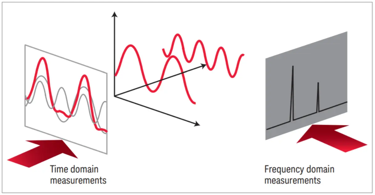
FFT works in the frequency domain, where each point represents a wave frequency rather than a world position. The FFT algorithm then converts the entire frequency domain into real world displacements (which live in the spatial domain) in one efficient pass. The beautiful thing about this, is that it’s a lossless operation. We can convert our data between domains without losing any information. This is neat since we can remove certain frequencies from the equation, convert the data back to the spatial domain and have the exact same wave minus the removed frequency. You can imagine this like having a musical chord, say C Major 7. This chord contains the notes C, E, G and B. Using the FFT, you would be able to see every note that this chord signal contains, remove the B for example and convert it back to the spatial domain. The result would be a simple C Major chord which has the notes C, E and G.
With this understanding of the FFT, we can now look at how Tessendorf uses it to build the ocean spectrum.

In his paper, Jerry Tessendorf describes the Phillips Spectrum as the model for defining wave energy. After implementing it I found it too limiting since its only parameters were wind speed and direction. So I switched to the JONSWAP spectrum, a more widely adopted model that gives much more creative freedom. With JONSWAP you can control things like how many waves follow the wind direction, the choppiness of the waves, the distance over which the wind affects the surface, and the sharpness of the spectrum peak. This lets you model anything from a calm open ocean to a stormy sea with large aggressive swells.

1.1 The Setup

The ocean simulation is driven by a statistical wave spectrum. Rather than simulating individual water particles, the sea surface is represented as a collection of many sinusoidal waves.

To simulate the ocean, the general idea is that we want to start by generating the initial representation of the heightfield in 2D space. We do this by using the wave spectrum in combination with a gaussian pseudo random number generator. The gaussian random number is used to ensure that each wave component starts at a different point in its cycle. This way two oceans with the same parameters will still look different from each other. This random number becomes the $\xi_r + i\xi_i$ term in the H₀ formula, which we will see in section 1.2.

Tessendorf expresses the ocean height field as a sum of complex wave contributions across all frequencies. We represent the ocean surface using the formula:

This heightfield is the result of the FFT converting the initial spectrum from the frequency domain to the spatial domain. This will be discussed in section 1.5. The complex amplitude $\tilde{h}(\mathbf{k}, t)$ is the heart of this formula. It is what we need to construct for every wave vector $\mathbf{k}$ on our grid. To do this we need two things: the JONSWAP spectrum, which tells us how much energy each wave frequency should carry, and the dispersion relation, which tells us how fast each wave travels. Section 1.3.

The dispersion relation allows us to propagate this heightfield forward in time, animating the waves. This will need to be recalculated every frame to update the heightfield accordingly. The dispersion relation defines the relationship between angular frequency $\omega$ and the wave number $k$.
In deep water, its formula is defined like this:

$\omega$ - Angular frequency. How fast the wave oscillates in time (radians/sec)
$g$ - Gravitational acceleration (9.81 m/s²)
$k$ - The Wavenumber. Waves per meter: $k = \frac{2\pi}{\lambda} $

For our implementation, we will be using the form that encodes a finite depth:

$D$ - Ocean Depth. Large values for D simplifies back to the base form while smaller values for D reduce the wave speed.

The dispersion relation formula is an approximation. There are many different relationships you can choose to fit your ocean.

With the general idea understood, we can now look at how the wave spectrum is constructed.

1.2 The Wave Spectrum

The wave spectrum is essentially a function that describes how the wave energy is distributed across combinations of angular frequencies $\omega$ and wind directions $\theta$.

The JONSWAP spectrum formula looks like this:

Before diving into each component of the JONSWAP, lets define a struct that will hold all the parameters that we will be populating.

	struct JonswapParameters
	{
		float scale = 0.0f; // Used to scale the Spectrum [1.0f, 5.0f] 
		float spreadBlend = 0.0f; // Used to blend between agitated water motion, and windDirection [0.0f, 1.0f]
		float swell = 0.0f; // Influences wave choppiness, the bigger the swell, the longer the wave length [0.0f, 1.0f]
		float gamma = 0.0f; // Defines the Spectrum Peak [0.0f, 7.0f]
		float shortWavesFade = 0.0f; // [0.0f, 1.0f]

		float windDirection = 0.0f; // [0.0f, 360.0f]
		float fetch = 0.0f; // Distance over which Wind impacts Wave Formation [0.0f, 10000.0f]
		float windSpeed = 0.0f; // [0.0f, 100.0f]

        // These values get calculated using the metrics above.
		float angle = 0.0f;
		float alpha = 0.0f;
		float peakOmega = 0.0f;
	}m_jonswapParams;

In code, calculating the JONSWAP spectrum looks like this:

float Ocean::JONSWAP(float omega)
{
    float sigma = (omega <= m_jonswapParams.peakOmega) ? 0.07f : 0.09f; // width parameter
    float r = exp(-(omega - m_jonswapParams.peakOmega) * (omega - m_jonswapParams.peakOmega) / 2.0f / sigma / sigma / m_jonswapParams.peakOmega / m_jonswapParams.peakOmega); // peak enhancement
    float g = 9.81f; // gravity

    float oneOverOmega = 1.0f / (omega + 1e-6f);
    float peakOmegaOverOmega = m_jonswapParams.peakOmega / omega;

    return m_jonswapParams.scale * TMACorrection(omega) * m_jonswapParams.alpha * g * g * oneOverOmega * oneOverOmega * oneOverOmega * oneOverOmega * oneOverOmega 
			* exp(-1.25f * peakOmegaOverOmega * peakOmegaOverOmega * peakOmegaOverOmega * peakOmegaOverOmega) * pow(abs(m_jonswapParams.gamma), r);
}

The TMA (Texel Marsen Arsloe) correction is used for the non directional component of the wave spectrum. This means that it does not care about the direction the waves are moving, instead the TMA functions on the depth of the ocean. In shallow waters, the seabed starts to intervene with the waves. The waves slow down, their shape changes and their energy distribution across waves get shifted. TMA accounts for this and adjusts the JONSWAP spectrum by multiplying the spectrum with a depth dependent factor.

float TMACorrection(float w)
{
    float omegaH = omega * sqrt(OCEAN_DEPTH / 9.81f);
    if (omegaH <= 1.0f)
        return 0.5f * omegaH * omegaH;
    if (omegaH < 2.0f)
        return 1.0f - 0.5f * (2.0f - omegaH) * (2.0f - omegaH);

    return 1.0f;
}

Before we continue, lets populate our JonswapParameters. I recommend you play with the values to meet your desired artistic vision.
We do need to calculate 3 of the variables: The angle, the alpha and the peakOmega.

m_jonswapParams.angle = m_jonswapParams.windDirection / 180.0f * PI;
m_jonswapParams.alpha = JonswapAlpha(m_jonswapParams.fetch, m_jonswapParams.windSpeed);
m_jonswapParams.peakOmega = JonswapPeakFequency(m_jonswapParams.fetch, m_jonswapParams.windSpeed);

float Ocean::JonswapAlpha(float fetch, float windSpeed)
{
    return 0.076f * pow(9.81f * fetch / windSpeed / windSpeed, - 0.22f);
}

float Ocean::JonswapPeakFequency(float fetch, float windSpeed)
{
    return 22.0f * pow(windSpeed * fetch / 9.81f / 9.81f, -0.33f);
}

Now that we have the wave spectrum, we can look at generating the initial heightfield.

1.3 Initial Spectrum Generation: H₀

We compute the initial spectrum once, my implementation does this on the CPU but its best done on the GPU since it can make great use of parallel computing.

The formula Tessendorf proposes in his paper is:

This data lives in the frequency domain.
We generate a complex number that encodes the amplitude and phase for every wave vector k. We store the resulting data in a R16G16B16A16_FLOAT texture.

Lets look at some code.

void Ocean::GenerateH0(std::shared_ptr<CommandList> commandList, const UINT cascade) {

    float deltaK = 2.0f * PI / patchSize;
    float highestK = (OCEAN_SUBRES / 2.0f) * deltaK; // nyquist limit

    // stored in heap to avoid stack overflow
    std::vector<std::complex<float>> H0(OCEAN_SUBRES * OCEAN_SUBRES, { 0,0 });
    std::vector<std::complex<float>> H0Conj(OCEAN_SUBRES * OCEAN_SUBRES, { 0,0 });

    const float lowCutoff = cascade == 0 ? 0.001f : (OCEAN_SUBRES * PI / m_oceanPatchSizes[cascade - 1]); // nyquist limit of previous cascade;
    const float highCutoff = highestK;
    
    
    for (int m = 0; m < OCEAN_SUBRES; m++) {
        for (int n = 0; n < OCEAN_SUBRES; n++) {
            // Get wave vector for this frequency
            float kx = (n - OCEAN_SUBRES / 2.0f) * deltaK;
            float ky = (m - OCEAN_SUBRES / 2.0f) * deltaK;
            float k(sqrtf(kx * kx + ky * ky));

            if (k >= lowCutoff && k <= highCutoff)
            {
	            
            float kAngle = atan2(ky, kx);
            float omega = DispersionRelation(k);
            float dOmegadk = DispersionDerivative(k);

            float spectrum = JONSWAP(omega) * DirectionSpectrum(kAngle, omega) * ShortWavesFade(k);
            
            // Generate two independent gaussian random numbers
            float xiR = GaussianRandom();
            float xiI = GaussianRandom();

            float amplitude = sqrtf(2.0f * spectrum * fabsf(dOmegadk) / k * deltaK * deltaK);
            H0[m * OCEAN_SUBRES + n] = std::complex<float>(xiR * amplitude, xiI * amplitude);
            }
        }
    }

    // Needs its own loop since the conjugate needs all data of H0 to be valid
    for (int m = 0; m < OCEAN_SUBRES; m++) {
        for (int n = 0; n < OCEAN_SUBRES; n++) {
            int m_minus = (OCEAN_SUBRES - m) % OCEAN_SUBRES;
            int n_minus = (OCEAN_SUBRES - n) % OCEAN_SUBRES;
            H0Conj[m * OCEAN_SUBRES + n] = std::conj(H0[m_minus * OCEAN_SUBRES + n_minus]);
        }
    }

    std::vector<uint16_t> combinedData(OCEAN_SUBRES * OCEAN_SUBRES * 4);

    for (int m = 0; m < OCEAN_SUBRES; m++) {
        for (int n = 0; n < OCEAN_SUBRES; n++) {
            int index = (m * OCEAN_SUBRES + n) * 4;
            combinedData[index + 0] = FloatToHalf(H0[m * OCEAN_SUBRES + n].real());       // R: H0 real
            combinedData[index + 1] = FloatToHalf(H0[m * OCEAN_SUBRES + n].imag());       // G: H0 imaginary
            combinedData[index + 2] = FloatToHalf(H0Conj[m * OCEAN_SUBRES + n].real());   // B: H0_conj real
            combinedData[index + 3] = FloatToHalf(H0Conj[m * OCEAN_SUBRES + n].imag());   // A: H0_conj imaginary
        }
    }

    D3D12_SUBRESOURCE_DATA subData = {};
    subData.pData = combinedData.data();
    subData.RowPitch = OCEAN_SUBRES * 4 * sizeof(uint16_t); // 4 channels * 2 bytes
    subData.SlicePitch = subData.RowPitch * OCEAN_SUBRES;

    commandList->CopyTextureSubresource(m_oceanCascades[cascade].H0Texture, 0, 1, &subData);
}

Lets dissect this.
deltaK is the spacing between frequency samples. Since our patch covers patchSize metres in the real world, dividing $2\pi$ by it gives us the step size in frequency space.
highestK is the Nyquist limit, the highest frequency our grid can represent before aliasing occurs.
lowCutoff and highCutoff can be ignored for now, these will be explained in Chapter 4.

The double for loop
For each grid position $(n, m)$ we compute the wave vector components kx and ky. Subtracting OCEAN_SUBRES / 2.0f centers the grid around zero so we cover both positive and negative frequencies, representing waves travelling in all directions.
k is the magnitude of the wave vector, the wavenumber.

Computing the spectrum value
For each wave vector we compute three things.
kAngle is the direction the wave is travelling.
omega is the angular frequency from the dispersion relation.
The full spectrum value is then the product of three functions. JONSWAP gives the total energy at this frequency.
DirectionSpectrum distributes that energy across directions based on kAngle.
ShortWavesFade damps out very high frequencies to prevent aliasing artifacts.

float SpreadPower(float omega, float peakOmega)
{
    if (omega > peakOmega)
        return 9.77f * pow(abs(omega / peakOmega), -2.5f);
    else
        return 6.97f * pow(abs(omega / peakOmega), 5.0f);
}

return lerp(
    2.0f / PI * cos(theta) * cos(theta),  // simple cosine squared, no directionality
    Cosine2s(theta - angle, s),            // full Hasselmann + swell spreading
    spreadBlend
);

Computing the amplitude and storing H₀ Two independent Gaussian random numbers give each wave component a unique random phase. The amplitude formula converts the continuous spectrum density into a discrete amplitude value for this specific grid cell, accounting for the cell size deltaK * deltaK. Multiplying the random numbers by the amplitude gives us $\tilde{h}_0(\mathbf{k})$, stored as a unique complex number.

The Conjugate
The conjugate is simply the sign mirror of a complex number. For example the conjugate of $z = a + bi$ is $z = a - bi$. This conjugate is needed since the FFT takes complex numbers as input and produces a complex number as an output too. Our heightfield needs to use real numbers, so using the conjugate we can cancel out the imaginary part of the FFT output, leaving us with only real values. for example:

Texture Packing
Both H0 and its conjugate are packed into a single RGBA texture. The real and imaginary parts of H0 go into the R and G channels, the conjugate goes into B and A. The values are converted to 16 bit half precision floats to save memory. This texture is then uploaded to the GPU where the compute shader will read it every frame to propagate the waves forward in time.

This function provides us with the initial spectrum texture. You can visualize this texture in your preferred graphics debugger, I’m using RenderDoc. You will need to change the color range to a very small value to see the colors clearly.

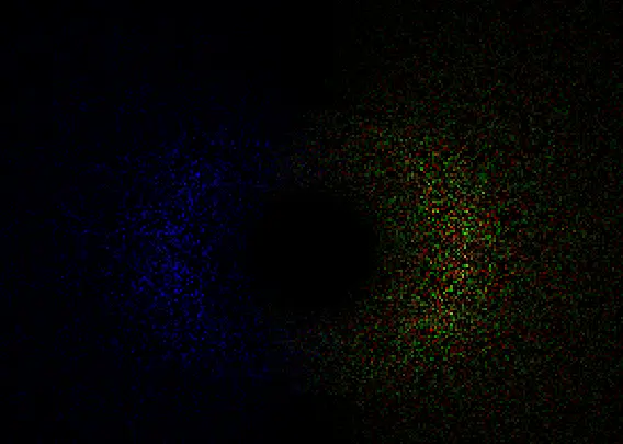
Your version might look slightly less colorful, mine is using multiple frequency bands which will be covered in Chapter 4.

Next we will look at how the FFT transforms this frequency domain data into real world wave displacements

1.4 Time Evolution: Animating the Waves

The next step now that we have the initial spectrum, is to bring our static data to life by animating it over time. Tessendorf provides us with the following formula:

Every frame, we take our initial spectrum $\tilde{h}_0(\mathbf{k})$ and multiply it by $e^{i\omega t}$. From Euler’s formula we know that this advances the phase of each wave component forward in time at its own speed, determined by the dispersion relation. The second term $\tilde{h}_0^*(-\mathbf{k})\,e^{-i\omega(k)t}$ is the conjugate we discussed earlier, ensuring the output remains a real value.

One important detail is that we use a rounded version of $\omega$ when computing the time evolution. This ensures that every wave component completes full cycles within a fixed time period, so the ocean animation loops seamlessly without any visible discontinuity.

So we have the initial spectrum and its conjugate, the last missing term is the dispersion relation and the $e^{i\omega t}$ which we will calculate now.
Since we want to loop the animation, we need to introduce a new variable: REPEAT_TIME. Using this variable we can control the amount of time it takes for the simulation to loop back to its original state. I’m using a value of 500 but feel free to play around with this.

First we load our initial spectrum and conjugate data.

float4 H0Data = H0Texture.Load(int3(dispatchThreadID.xy, 0));
float2 h0 = H0Data.rg;
float2 h0conj = H0Data.ba;

float kx = 2.0f * PI * (dispatchThreadID.x - OCEAN_RESOLUTION / 2.0f) / patchSize;
float ky = 2.0f * PI * (dispatchThreadID.y - OCEAN_RESOLUTION / 2.0f) / patchSize;
float k = length(float2(kx,ky));
float kRcp = rcp(k);

// Prevent NaN values
if (k < 0.0001f)
{
    kRcp = 1.0f;
}

We calculate the base frequency step.

float w = 2.0f * PI / REPEAT_TIME;

We can use this value as the stepsize around the unit circle and use time as the scalar that advances the dispersion.

float dispersion = floor(sqrt(GRAVITY * k) / w) * w * time;

We now plug this dispersion into Euler’s formula which gives us $e^{i\omega t}$. Add these helper functions:

float2 EulerFormula(float x)
{
    return float2(cos(x), sin(x));
}

float2 complex_multiply(float2 W, float2 B)
{
    return float2(W.x * B.x - W.y * B.y,
                  W.x * B.y + W.y * B.x);
}

float2 exponent = EulerFormula(dispersion);

Now we have all the components to calculate $\tilde{h}(\mathbf{k}, t)$

float2 htilde = complex_multiply(h0, exponent) + complex_multiply(h0conj, float2(exponent.x, -exponent.y));

We now successfully computed the heightfield in the frequency domain. Next to this, we also want to have the horizontal displacement and the surface slope. The horizontal displacement will make the waves look choppy and the slopes are used to calculate the surface normals which we will be using in Chapter 2 for lighting calculations.

From the animated spectrum $\tilde{h}(\mathbf{k}, t)$ we can derive everything we need in one pass. Rather than running separate FFTs for height, horizontal displacement and surface slopes, we compute all of them in the frequency domain before the FFT using a property of Fourier transforms: taking a spatial derivative in the real world is equivalent to multiplying by $ik$ in the frequency domain.

First we precompute $i\tilde{h}$, which is just the complex number rotated 90 degrees:

float2 ih = float2(-htilde.y, htilde.x);

Then we derive each output signal:

// the raw height field, becomes vertical displacement after the FFT
float2 displacementY = htilde;
// horizontal displacement in x and z, pointing in the wave travel direction
float2 displacementX = ih * kx * kRcp;
float2 displacementZ = ih * ky * kRcp;
// the surface slopes in x and z, used to compute normals for lighting
float2 displacementY_dx = ih * kx;
float2 displacementY_dz = ih * ky;
// second order derivatives used to compute the Jacobian determinant for foam detection. Covered in Chapter 3. 
float2 displacementZ_dx = -htilde * kx * ky * kRcp;
float2 displacementZ_dz = -htilde * ky * ky * kRcp;
float2 displacementX_dx = -htilde * kx * kx * kRcp;

The negative sign on the second order derivatives comes from applying the $ik$ multiplication twice: $i^2 = -1$, so $ik \cdot ik = -k^2$.

All eight signals are then packed into two float4 textures and converted to the spatial domain by the FFT in the next pass.

float2 htildeDisplacementX = float2(displacementX.x - displacementZ.y, displacementX.y + displacementZ.x);
float2 htildeDisplacementZ = float2(displacementY.x - displacementZ_dx.y, displacementY.y + displacementZ_dx.x);
    
float2 htildeSlopeX = float2(displacementY_dx.x - displacementY_dz.y, displacementY_dx.y + displacementY_dz.x);
float2 htildeSlopeZ = float2(displacementX_dx.x - displacementZ_dz.y, displacementX_dx.y + displacementZ_dz.x);


displacementTexture[dispatchThreadID.xy] = float4(htildeDisplacementX, htildeDisplacementZ);
slopeTexture[dispatchThreadID.xy] = float4(htildeSlopeX, htildeSlopeZ);

With this, we now have the heightfield, horizontal displacement and slopes, all calculated in the frequency domain. The last step is to transform this data to the spatial domain.

1.5 The Butterfly FFT

Understanding the FFT

The ocean simulation depends on converting a frequency domain wave spectrum into real displacement values every frame. That conversion is an Inverse Fast Fourier Transform. In this section I will explain the idea behind this transformation and how it works. To not make this article too long/complex, I will not go too much into detail since understanding it fully is not required to make it work. If you are brave enough you can dive deeper and read the paper by Flugge and Matusiak.

float angle = -2.0f * PI * float(w) / float(TOTALPOINTS);
float2 twiddle = float2(cos(angle), -sin(angle));

for (uint stage = 0; stage < log2(TOTALPOINTS); ++stage)

groupshared float2 bufferRG[2][TOTALPOINTS];
groupshared float2 bufferBA[2][TOTALPOINTS];

uint flag = 0;
for (uint stage = 0; stage < log2(TOTALPOINTS); ++stage)
{
    bufferRG[1 - flag][groupIndex] = bufferRG[flag][i] + complex_multiply(twiddle, bufferRG[flag][i + b]);
    flag = 1 - flag;
    GroupMemoryBarrierWithGroupSync();
}

uint b = TOTALPOINTS >> (stage + 1);
uint w = b * (groupIndex / b);
uint i = (w + groupIndex) % TOTALPOINTS;

if (columnPass)
    data = outputTexture.Load(int3(groupID.x, groupIndex, 0));
else
    data = outputTexture.Load(int3(groupIndex, groupID.x, 0));

groupshared float2 bufferRG[2][TOTALPOINTS];
groupshared float2 bufferBA[2][TOTALPOINTS];

[numthreads(TOTALPOINTS, 1, 1)]
void main(uint3 dispatchThreadID : SV_DispatchThreadID, uint3 groupID : SV_GroupID, uint groupIndex : SV_GroupIndex)
{
    float4 data;
    if (columnPass)
        data = outputTexture.Load(int3(groupID.x, groupIndex, 0)); // column: x fixed, y varies
    else
        data = outputTexture.Load(int3(groupIndex, groupID.x, 0)); // row: x varies, y fixed

    bufferRG[0][groupIndex] = data.rg;
    bufferBA[0][groupIndex] = data.ba;

    GroupMemoryBarrierWithGroupSync();
    
    uint flag = 0;
    for (uint stage = 0; stage < log2(TOTALPOINTS); ++stage)
    {
        uint b = TOTALPOINTS >> (stage + 1);
        uint w = b * (groupIndex / b);
        uint i = (w + groupIndex) % TOTALPOINTS;

        float angle = -2.0f * PI * float(w) / float(TOTALPOINTS);
        float2 twiddle = float2(cos(angle), -sin(angle));

        bufferRG[1 - flag][groupIndex] = bufferRG[flag][i] + complex_multiply(twiddle, bufferRG[flag][i + b]);
        bufferBA[1 - flag][groupIndex] = bufferBA[flag][i] + complex_multiply(twiddle, bufferBA[flag][i + b]);

        flag = 1 - flag;
        GroupMemoryBarrierWithGroupSync();
    }

    float2 resultRG = bufferRG[flag][groupIndex];
    float2 resultBA = bufferBA[flag][groupIndex];

    if (columnPass)
        outputTexture[int2(groupID.x, groupIndex)] = float4(resultRG, resultBA);
    else
        outputTexture[int2(groupIndex, groupID.x)] = float4(resultRG, resultBA);
}

Putting all this together, after both passes complete we have converted our wave spectrum from the frequency domain into real spatial data. Before we can use this data to displace our vertices, we need to apply one last step to correctly arrange it.

Permuting the FFT Output

Before we can use the FFT results, we need to apply two final steps: centering the output and unpacking our signals.

Centering the spectrum

The raw FFT output places the zero frequency component in the corner of the texture. For our ocean patch this means the waves are arranged awkwardly, with the lowest frequencies split across opposite corners. We fix this by the following permute function:

float4 Permute(float4 data, float3 id)
{
    return data * (1.0f - 2.0f * ((id.x + id.y) % 2));
}

This flips the sign of every other texel in a checkerboard pattern, which has the effect of shifting the zero frequency component from the corner to the center. After this step the wave frequencies are arranged symmetrically, which is what we need for a correct tileable patch.

Unpacking the signals

Back in the wave animation pass we packed multiple signals into two float4 textures to save GPU passes. Now we unpack them:

float2 dxdz   = htildeDisplacement.rg;  // horizontal displacement in X and Z
float2 dydxz  = htildeDisplacement.ba;  // vertical displacement Y, and the Dxz cross derivative
float2 dyxdyz = htildeSlope.rg;         // surface slopes in X and Z, used for normals
float2 dxxdzz = htildeSlope.ba;         // second derivatives Dxx and Dzz, used for the Jacobian (Expanded upon in Chapter 3)

Applying choppiness

The horizontal displacements are scaled by a factor called Lambda before being applied to the mesh. Lambda controls how choppy the waves look. A value of 0 gives smooth rolling swells, higher values push the wave crests forward to create the sharp peaked shapes you see on a real ocean surface.

float3 displacement = float3(Lambda.x * dxdz.x, dydxz.x, Lambda.y * dxdz.y);

The slopes used for normal calculation get a Lambda correction too. In areas of strong horizontal displacement the surface is being stretched and compressed, which would cause the normal map to produce incorrect results without accounting for it:

float2 slopes = dyxdyz.xy / (1 + abs(dxxdzz * Lambda));

Finally we store this data in their corresponding textures:

slopeTexture[dispatchThreadID.xy] = float4(slopes, 0.0f, 1.0f);
displacementTexture[dispatchThreadID.xy] = float4(displacement, 0.0f);

With this, the hard part is behind us. Take a look at the contents of the texture, it should look something like this:

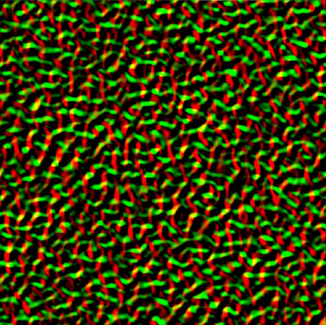
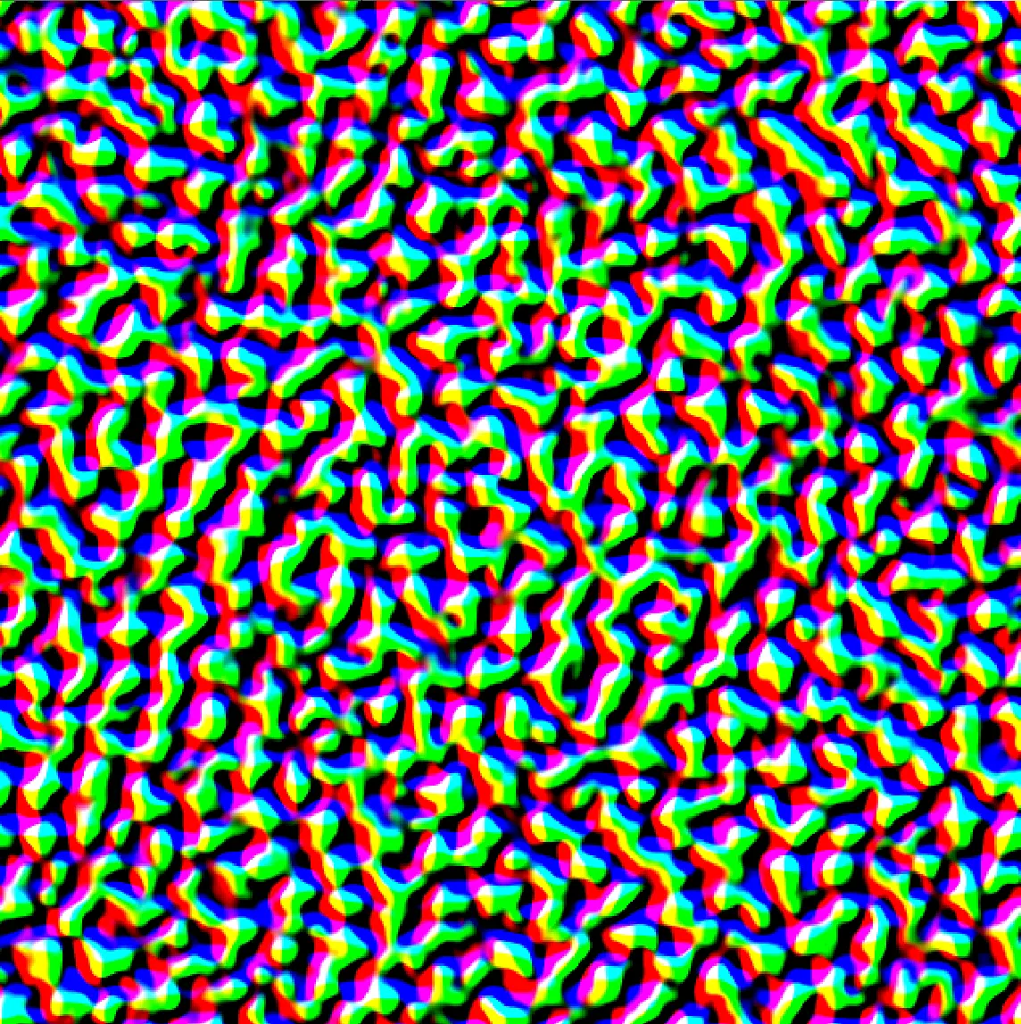
You’ve succesfully created the slope and displacement textures! In the next chapter I will show you how to use these textures to render the Ocean.

References

1. Tessendorf, J. (2001). Simulating Ocean Water. SIGGRAPH Course Notes.
2. Christopher J. Horvath
3. [GarrettGunnell.] (https://github.com/GarrettGunnell/Water). GitHub.
4. [gasgiant.] (https://github.com/gasgiant/FFT-Ocean). GitHub.
5. Fynn-Jorin Flügge.
6. Bolba, G. Ocean rendering blog post.

About Timethy Hyman

Timethy, an aspiring grahics programmer.

Email : timethy.hyman@gmail.com